A simple power supply
Getting started
In this example, we will analyze a simple power supply.
The power supply consists of a “lump” power transformer with fairly loose coupling for short circuit protection, a full wave bridge rectifier, and a filter capacitor. The desired output is about 50 volts at .5 amps (100 Ohm load), with less than 1 volt of ripple. The power supply should be able to handle a short with no damage, with no fuse.
An inexperienced engineer has chosen a transformer with primary inductance of 1 Henry, secondary inductance of .1 Henry, a turns ratio of 3.16:1. The stock transformer has a coefficient of coupling of .9. He has also chosen 1N4004 diodes, and a 5000 uf filter capacitor.
The first goal of simulation is to validate the design. Then, make adjustments to the design to meet the specs.
To validate the design, the following measurements need to be made, not necessarily in this order.
- DC output voltage, loaded (100 Ohm) and unloaded.
- Ripple voltage.
- Current in diodes: waveform, average, steady state peak, power-on surge, AC.
- Current in filter cap: as above
- Input current: as above
- Input power, VAR, and power factor: as above
- Above currents and power for load = nominal (100 Ohm), unloaded, and shorted (.01 Ohm)
- Diode voltages, PIV, etc.
- Transformer voltages
- Impact of high line (132 volts) and low line (108 volts)
This example will show how to do some of these. The rest are left as an exercise. You can make all of these measurements with gnucap.
Building the circuit
Models
First, let's make subcircuits for the transformer and diode bridge:
.subckt transformer (p1 p2 s1 s2)
L1 (p1 p2) 1
L2 (s1 s2) .1
K1 (L1 L2) .9
.ends

.subckt bridge (in1 in2 minus plus)
.model 1n4004 d is=1n
D1 (in1 plus) 1n4004
D2 (in2 plus) 1n4004
D3 (minus in1) 1n4004
D4 (minus in2) 1n4004
.ends
Save it in the file “models”.
Main circuit
Now, let's run it interactively.. Type in the circuit…
$ gnucap
..... (signs on)
gnucap> include models
gnucap> list
   ..... (list of circuit so far)
gnucap> spice
gnucap-spice>Vin (in 0) sin (freq=60 ampl=170) ac 120
gnucap-spice>X1 (in 0 s1 s2) transformer
gnucap-spice>X2 (s1 s2 0 out) bridge
gnucap-spice>R1 (s1 0) 10k
gnucap-spice>R2 (s2 0) 10k
gnucap-spice>Rload (out 0) rload
gnucap-spice>Cfilter (out 0) cfilter
gnucap-spice>.control
gnucap>
Note the two extra resistors R1, R2. These will tie down the nodes s1 and s2 during the input polarity flip, when the diodes are all open.
Simulate
Try
gnucap> param cfilter 5000u
gnucap> param rload 100
gnucap> print tran v(nodes)
gnucap> tr .2 trace=a > tr.out
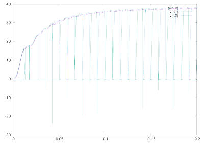
Now, there is a file tr.out with voltages over time. Plot some of it, and it may look like
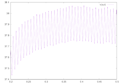
We are interested in v(out). Store it from now on, and simulate a bit further.
gnucap> store tran v(out)
gnucap> tr .5 trace=a > tr.out
OK, not perfect. We should have waited until .3 or more for it to settle. Try tr 0 .3 if you are curious. Anyway, with this waveform stored, we can do some measurements as follows.
gnucap> measure min=min("v(out)")
min= 37.4370112192329
gnucap> measure max=max("v(out)")
max= 38.0723316837578
gnucap> param range = max-min
gnucap> eval range
range= 0.635320464524902
gnucap> measure mean=mean("v(out)")
mean= 37.8378453386751

